How to Control Robot Arms: Kinematics, Dynamics, and Force Feedback
Controlling a robot arm requires mastering kinematics, dynamics, and feedback control. This guide covers forward/inverse kinematics, Jacobians, PID control, and force feedback for manipulation.
Introduction
Controlling a robot arm requires mastering kinematics, dynamics, and feedback control. This guide covers forward/inverse kinematics, Jacobians, PID control, and force feedback for manipulation.
Prerequisites
- ✓ Linear algebra (matrices, transformations)
- ✓ Calculus (derivatives)
- ✓ Python or C++ programming
- ✓ Basic ROS2 knowledge
Key Concepts
Step-by-Step Guide
- 1
Understand Robot Arm Kinematics
A robot arm is a chain of links connected by joints. Each joint adds one DOF. A 6-DOF arm can reach any position and orientation. Forward kinematics computes end-effector position from joint angles (matrix multiplication). Inverse kinematics computes joint angles for a target position — harder, may have multiple solutions.
python# Forward kinematics using DH parameters import numpy as np def dh_transform(theta, d, a, alpha): return np.array([ [np.cos(theta), -np.sin(theta)*np.cos(alpha), np.sin(theta)*np.sin(alpha), a*np.cos(theta)], [np.sin(theta), np.cos(theta)*np.cos(alpha), -np.cos(theta)*np.sin(alpha), a*np.sin(theta)], [0, np.sin(alpha), np.cos(alpha), d], [0, 0, 0, 1]]) def fk_2dof(theta1, theta2, l1, l2): T1 = dh_transform(theta1, 0, l1, 0) T2 = dh_transform(theta2, 0, l2, 0) return (T1 @ T2)[:2, 3] - 2
Master DH Parameters
DH parameters describe robot arm geometry: theta (joint angle), d (link offset), a (link length), alpha (link twist). Assign frames to each link following DH conventions, then build the transformation chain.
Tip: Use modified DH parameters (Craig convention) — more intuitive and widely used in modern robotics textbooks. - 3
Solve Inverse Kinematics
IK finds joint angles for a target. Analytical solutions exist for simple arms (2-DOF planar) and 6-DOF arms with spherical wrists. For general cases, use numerical methods: Jacobian pseudo-inverse, CCD, or TRAC-IK. MoveIt2 provides production-ready IK.
python# Analytical IK for 2-DOF planar arm import numpy as np def ik_2dof(x, y, l1, l2): c2 = (x**2 + y**2 - l1**2 - l2**2) / (2*l1*l2) if abs(c2) > 1: raise ValueError("Out of reach") t2 = np.arccos(c2) t1 = np.arctan2(y, x) - np.arctan2(l2*np.sin(t2), l1+l2*np.cos(t2)) return t1, t2 - 4
Understand the Jacobian
The Jacobian J maps joint velocities to end-effector velocities: ẋ = J·θ̇. Used for velocity control, force transformation (τ = Jᵀ·F), and singularity detection (det(J)=0). Singularities occur when the arm loses a DOF.
Warning: Near singularities, small Cartesian velocities require huge joint velocities. Use damped least-squares (DLS) inverse for numerical stability. - 5
Implement PID Position Control
PID control drives each joint motor to track a desired position. P reduces rise time, I eliminates steady-state error, D reduces overshoot. For robot arms, cascaded PID (position → velocity → torque) provides better performance.
pythonclass PID: def __init__(self, kp, ki, kd): self.kp, self.ki, self.kd = kp, ki, kd self.integral = 0 self.prev_error = 0 def update(self, setpoint, measurement, dt): error = setpoint - measurement self.integral += error * dt deriv = (error - self.prev_error) / dt self.prev_error = error return self.kp*error + self.ki*self.integral + self.kd*deriv - 6
Generate and Track Trajectories
Trajectory generation creates smooth motion between waypoints: polynomial interpolation (quintic for smooth velocity/acceleration), trapezoidal velocity profiles, B-splines. Use computed torque control or PID feedback for tracking. MoveIt2 handles trajectory generation and collision checking.
Tip: Use quintic polynomial interpolation — continuous position, velocity, and acceleration, minimizing jerk and reducing joint wear. - 7
Implement Force/Torque Control
Position control cannot handle contact tasks (assembly, polishing). Force control regulates contact force. Hybrid force/position control: force in constrained directions, position in free directions. Impedance control: arm behaves like a spring-damper. Force/torque sensors (ATI, OnRobot) measure contact forces.
Surgical robots use force feedback to let surgeons feel tissue resistance — demonstrating force control in delicate manipulation. - 8
Use MoveIt2 for Motion Planning
MoveIt2 is the standard ROS2 motion planning framework: IK solvers, OMPL planning, FCL collision checking, trajectory execution, RViz2 visualization. Configure with your URDF, then use the MoveGroup action interface.
python# MoveIt2 Python interface import rclpy from moveit.planning import MoveItPy rclpy.init() moveit = MoveItPy(node_name="moveit_py") arm = moveit.get_planning_component("arm") arm.set_pose_target([0.3, 0.2, 0.5, 0.0, 0.0, 0.0]) plan = arm.plan() if plan.planning_result.success: arm.execute(plan.trajectory) - 9
Implement Compliant Control
Compliant control makes arms safe for human interaction. Admittance control: measure force, compute position offset, command to position controller. Impedance control: regulate force-motion relationship. Variable stiffness: adjust compliance by task phase. Essential for cobots.
Warning: Industrial robots with high stiffness and no force sensing are dangerous to humans. Cobots (UR, Franka, KUKA iiwa) use torque sensors and compliant control for safe collaboration. - 10
Calibrate and Identify Dynamics
Dynamic model: τ = M(q)·q̈ + C(q,q̇)·q̇ + G(q) + F. M=inertia, C=Coriolis, G=gravity, F=friction. Accurate dynamics enable computed torque control and force estimation. Identify parameters via least-squares from trajectory data.
textRobot Arm Dynamics: τ = M(q)·q̈ + C(q,q̇)·q̇ + G(q) + F(q̇) M: inertia matrix, C: Coriolis, G: gravity, F: friction Computed Torque: τ = M(q)·(q̈_d + Kp·e + Kd·ė) + C·q̇ + G - 11
Integrate Grasping
Gripper types: parallel jaw (reliable), vacuum (fast, flat objects), soft (adaptive, fragile). Grasp planning: antipodal grasping, Dex-Net database, GraspNet deep learning. Pipeline: approach, grasp, lift, transport, place.

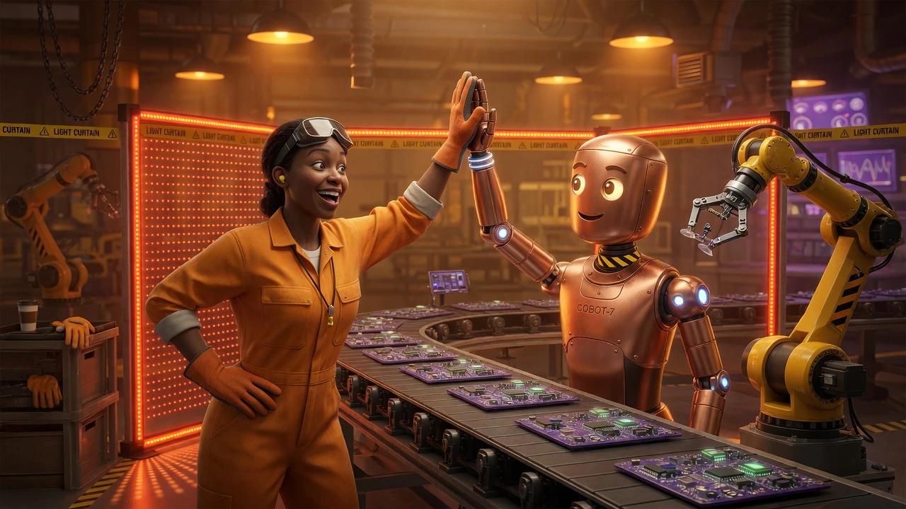
A cobot performing assembly — arm control, force feedback, and grasping integrated into a complete manipulation pipeline. - 12
Deploy to a Real Robot
Simulation to real requires: accurate URDF, calibrated kinematics, tuned PID gains, safety limits. Use ros2_control for hardware abstraction. Start with 10% speed and increase gradually.
Warning: Never deploy without testing in simulation first (Gazebo, Isaac Sim). Verify joint limits, collision avoidance, and e-stop. A controller bug can cause violent motion.
Summary
Robot arm control requires kinematics (FK: angles→position, IK: position→angles), dynamics (forces/torques), and feedback control (PID). The Jacobian maps joint to Cartesian velocities and detects singularities. MoveIt2 provides production-ready motion planning. Force/torque control (impedance, admittance) is essential for contact tasks and safe human interaction.
Frequently Asked Questions
FK computes end-effector position from joint angles (straightforward). IK computes joint angles for a target position (harder, may have multiple/no solutions, often needs numerical methods).
A configuration where the robot loses a DOF — cannot move in a Cartesian direction. Jacobian determinant is zero. Near singularities, small Cartesian moves require huge joint velocities. Use damped least-squares IK.
Torque sensors enable force control, collision detection, and compliant behavior. Without force sensing, arms are stiff and dangerous. With torque sensing, arms detect contact, stop, and behave compliantly — safe for human workspaces.
Use MoveIt2 for production — battle-tested IK (TRAC-IK, KDL), OMPL planning, FCL collision checking. Only write custom for unusual mechanisms (cable-driven, soft robots).
Test Your Knowledge
1. What does the Jacobian matrix represent?
J maps joint velocities to end-effector velocities (ẋ = J·θ̇) and forces to torques (τ = Jᵀ·F). Its determinant indicates singularities.
2. Why is IK harder than FK?
FK is direct (multiply matrices). IK is an inverse problem — multiple configurations may reach the same position, or no solution exists for unreachable targets.
3. Purpose of impedance control?
Impedance control regulates the force-motion relationship, making the arm behave like a mass-spring-damper. Provides compliance for contact tasks and safe human interaction.